2 Operating Models
2.1 OM Conditioning
The operating models (OMs) were conditioned with an Approximate Bayesian Computation (ABC) approach (Section 2.1.1) developed for IOTC tuna species (Hillary & Mosqueira, 2024). The conditioning model outputs were downloaded from the albMSE GitHub repository and imported into the iotcALB framework.
The following specifications are common to all operating models:
Number of independent simulations: 500, from the ABC MCMC posterior samples;
Historical period: 2000–2020, with 4 quarterly time steps per year;
Population structure: two sexes (female and male), with quarterly age classes up to age 14 and recruitment in the fourth quarter.
NoteRobustness OMs
In the conditioning code available in the albMSE repository, the robustness OMs OM5a and OM6b appear to have been conditioned with the same index as the Base Case OM, without a catchability trend, so only the Base Case OM (OM5b) is projected in this MSE (Section 2.2).
2.1.1 Approximate Bayesian Computation (ABC) Model
The ABC approach generates a distribution of plausible historical stock dynamics that is consistent with available data and a set of prior beliefs about current and historical stock status.
The population model underlying the ABC conditioning mirrors the structure of the most 2022 Indian Ocean albacore stock assessment. The key structural features are:
- Annual age structure with four seasons per year and recruitment occurring in last quarter;
- Sex-structured population dynamics with sex-specific growth and weight-at-age;
- Six fleets: four longline fleets (LL1–LL4), a purse seine fleet, and an “other” fleet;
- A Beverton-Holt stock-recruit relationship with lognormally distributed recruitment deviations;
- Conditioning period: 2000–2020.
The ABC algorithm is implemented as an MCMC sampler (ABC-MCMC). The reported catches of each fleet and season are assumed to be known without error. The model is fitted to two data sources: the seasonal LL1 CPUE index and the length-frequency composition data of each fleet, pooled over all years and seasons.
2.1.2 Fleet Structure
To reduce run time, the six fleets of the ABC model were combined into a single aggregated fleet in the OMs. The combined fleet reproduces the historical fishing mortality-at-age of the individual fleets, with selectivity and weight-at-age weighted by the fishing mortality of each fleet, so the fishery and population dynamics are the same as an OM with the six fleets. In the projection period, the relative contribution of each fleet to the total catch is therefore assumed to be fixed at its recent pattern.
2.1.3 Indices of Abundance
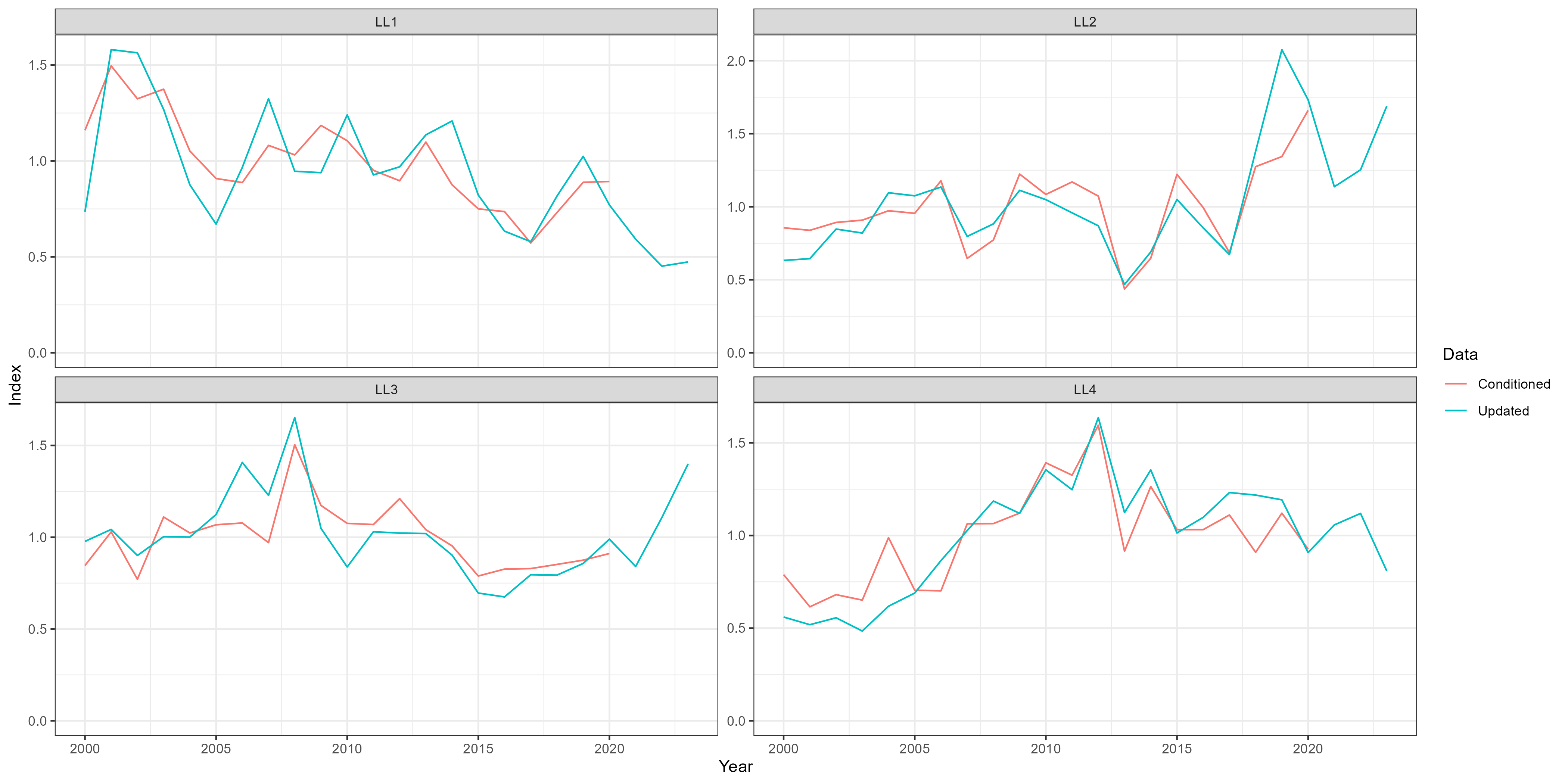
The ABC model includes seasonal CPUE indices for the four longline fleets (LL1–LL4; Figure 2.2). In the OMs these indices keep the selectivity of their respective fleet, so they continue to be simulated in the projection period as indices of the vulnerable biomass of the corresponding longline fleet (Chapter 3).
The Base Case OM is conditioned on the LL1 (NW) CPUE, the index used by the candidate management procedures (CMPs; Chapter 5). The other indices are not currently used by the CMPs.
2.1.4 Updated Fishery Data
The OMs are conditioned on the data assembled for the 2022 stock assessment (IOTC, 2022), with data up to 2020. Catch and CPUE data up to 2023 are now available from the 2025 stock assessment, including a revision of the historical catches and CPUE indices standardised with a revised methodology.
The current OMs have not been reconditioned to these data. Instead, the updated data are used in two ways:
- The reported catches in 2021–2023 are applied in the first years of the projection period (Section 3.2);
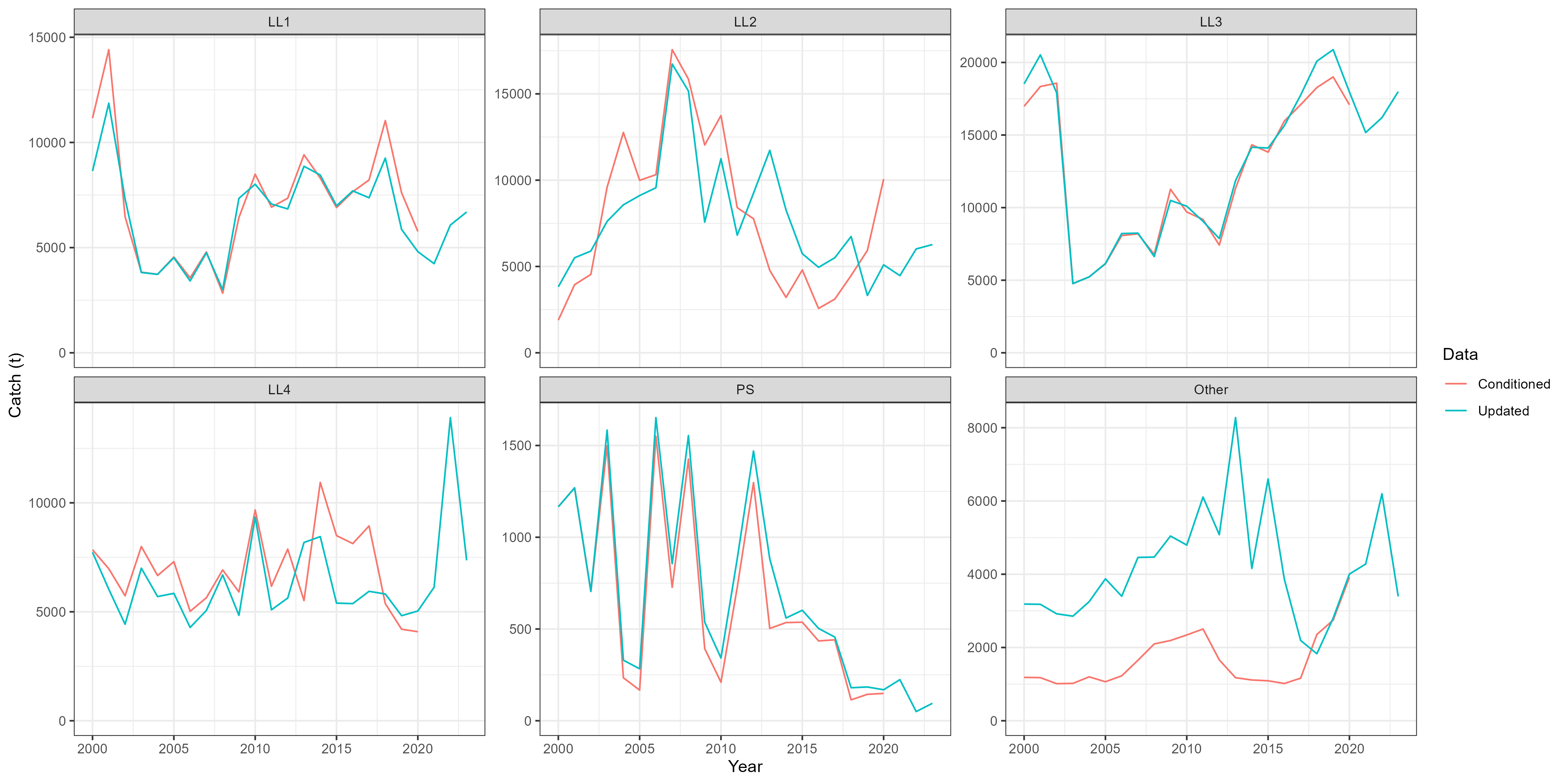
- The catch and CPUE data passed to the CMPs are replaced with the updated data for the historical period and for 2021–2023, so the CMPs use the current fishery data (Figure 2.1, Figure 2.2). The observation error of the simulated indices in the projection period is conditioned on the fit of the OM to the original CPUE series that the models were conditioned on (Chapter 3).
The updated LL1 CPUE declines more steeply over the last decade than the index used to condition the OMs, and the 2021–2023 values are on average 34% lower than the 2016–2020 mean. The OMs do not predict a decline of this magnitude for most simulations (Section 3.2.1).
The revised historical catches are similar to the catches used to condition the OMs on average (mean total catch over 2000–2020 of 38,200 t, compared with 36,600 t), with the largest revisions in 2013–2015 (up to 52% higher in 2013) and in the catches of the “Other” fleet, which are higher in the updated data over most of the period, while some of the longline catches appear to be reallocated among the longline fleets (Figure 2.1).
2.1.5 Additional Robustness OMs
Mosqueira & Hillary (2025) describe two additional robustness OMs:
-
OM5b_cc: the Base Case OM with climate change effects on recruitment, maturity, growth, and carrying capacity; -
OM5b_rec: an OM with sudden reductions in recruitment, with 25 and 50% lower recruitment deviations than the Base Case OM.
These OMs are not available in the albMSE GitHub repository and are not currently included in the MSE.
2.2 Review of the Conditioning
Importing the ABC conditioning model output into the iotcALB MSE framework identified some potential issues that may affect the population dynamics described in the OMs. It is possible that the albMSE repository does not include the latest version of the code and outputs, so some of these issues may already have been resolved.
These issues are summarised below and will be discussed with the members of the Working Party on Tropical Tunas and the authors of the conditioning model before any re-conditioning is run:
In the repository code, the robustness OMs
OM5aandOM6bappear to have been conditioned with the same index (LL1) as the Base Case OM (OM5b); i.e.,OM5awas not fit to the LL2 index andOM6bdoes not appear to include the catchability trend. In the current form,OM5aandOM6bdo not represent the alternative hypotheses they were designed for, and therefore only the Base Case OM (OM5b) is currently projected in MSE;In the MCMC sampler, steepness and natural mortality appear to be redrawn from their prior without an accept/reject step, so some of the stored posterior draws do not meet the length composition criterion when re-evaluated;
The ABC model uses a harvest rate (pulse fishing), while the OMs use the Baranov catch equation, which causes small differences between the OMs and the conditioning model (see Section 2.4).
Regardless of these issues, it is recommended that the OMs should be reconditioned, because data up to 2023 are now available, including revised historical catches and a revised CPUE standardisation (Section 2.1.4). In particular, the OMs do not predict the decline in the updated LL1 CPUE in 2021–2023, so the index simulated from 2024 is on average about twice the observed 2021–2023 index, an artificial increase in the data used by the CMPs (Section 3.4). The reconditioning would also be an opportunity to consider using the Baranov catch equation in the conditioning model, so that the OMs reproduce it exactly (see Section 2.4).
If the OMs are reconditioned, the CMPs will need to be re-tuned, so the current results should be interpreted with this in mind.
2.3 Historical Stock Status
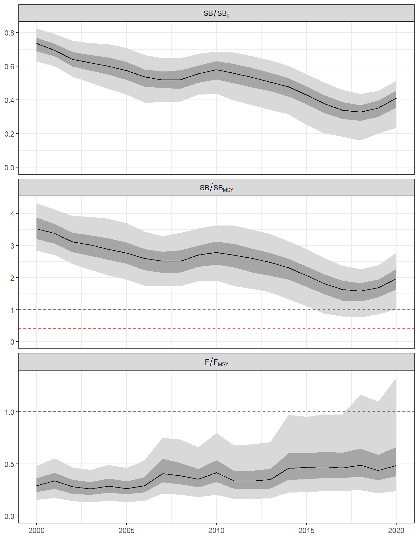
The stock status of the Base Case OM is reported for the female spawning biomass (SB) and the annual apical fishing mortality (F). Table 2.1 summarises the MSY reference points and the stock status in 2020, and Figure 2.3 shows the historical time series.
In 2020, the median spawning biomass was 0.41 SB0 and 1.96 SBMSY, and the median fishing mortality 0.49 FMSY. The stock was above SBMSY in 95% of simulations, and below the limit reference point in 1 of the 500 simulations. However, under the catches of the initial projection years (2021–2028), the stock is below the limit reference point in about 6% of simulations (30) by 2029, the first year of MP advice, mainly the low-productivity simulations (Section 3.2.1).
The IOTC reference points for albacore are defined relative to SBMSY and FMSY(IOTC, 2015). Because the longline fleets mainly catch mature fish and steepness is high, SBMSY is a small fraction of the unfished spawning biomass in the Base Case OM. On average, the target (SBMSY) corresponds to about 18% of SB0, and the limit reference point (0.4 SBMSY) to about 7.3% of SB0 (6.2–8.4%, 5th–95th percentiles; Table 2.1).
| Quantity | Median (5th–95th percentile) | |
|---|---|---|
| MSY reference points | MSY (t) | 51,055 (32,220–90,814) |
| FMSY | 0.48 (0.36–0.66) | |
| SBMSY (t) | 24,913 (15,791–44,957) | |
| Relative to unfished | SBMSY/SB0 | 0.183 (0.154–0.209) |
| 0.4 SBMSY/SB0 | 0.073 (0.062–0.084) | |
| Stock status in 2020 | SB/SB0 | 0.41 (0.23–0.51) |
| SB/SBMSY | 1.96 (1.00–2.77) | |
| F/FMSY | 0.49 (0.24–1.33) |
2.4 Differences Between the ABC Conditioning Model and the OMs
2.4.1 Harvest Rate vs. Instantaneous Fishing Mortality
The ABC model and the iotcALB OM differ in how they represent the removal of fish by fishing activity. This difference has implications for how the OM reproduces the stock dynamics of the conditioning model.
The ABC model uses a harvest rate approach, sometimes referred to as pulse fishing, while the iotcALB model uses the Baranov catch equation.
Under the harvest rate formulation, fishing occurs as a discrete pulse at the start of each time step: a fixed proportion \(H\) of the vulnerable population, as it stands at the start of the time step, is removed, after which natural mortality acts on the survivors for the remainder of the time step. The within-season dynamics are described as:
\[N_{t+1} = N_t \cdot \prod_f \left(1 - H_{f,t} \cdot s_{a,f}\right) \cdot e^{-M} \tag{2.1}\]
where \(s_{a,f}\) is the age- and fleet-specific selectivity and \(M\) is the instantaneous natural mortality rate. Catch by fleet is:
\[C_{f,t} = N_t \cdot H_{f,t} \cdot s_{a,f} \tag{2.2}\]
The Baranov catch equation approach assumes fishing and natural mortality act simultaneously and continuously throughout the time step. Total mortality \(Z\) is:
\[Z_t = M + \sum_f F_{f,t} \cdot s_{a,f} \tag{2.3}\]
and catch by fleet is:
\[C_{f,t} = N_t \cdot \frac{F_{f,t} \cdot s_{a,f}}{Z_t} \cdot \left(1 - e^{-Z_t}\right) \tag{2.4}\]
To import the ABC output into iotcALB, fleet-specific harvest rates are converted to instantaneous fishing mortality as:
\[F_f = -\log(1 - H_f) \tag{2.5}\]
While this conversion is exact in a mathematical sense, the two formulations differ in how total mortality is partitioned between fishing and natural causes. Under the pulse fishing formulation, the full harvest rate \(H_f\) is applied to the population at the start of the time step, and natural mortality then acts on the survivors (Equation 2.2). Under the Baranov equation, fishing and natural mortality act simultaneously, so a larger share of total mortality is attributed to natural causes and a correspondingly smaller share to fishing (Equation 2.4).
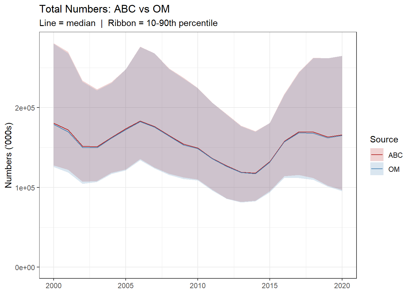
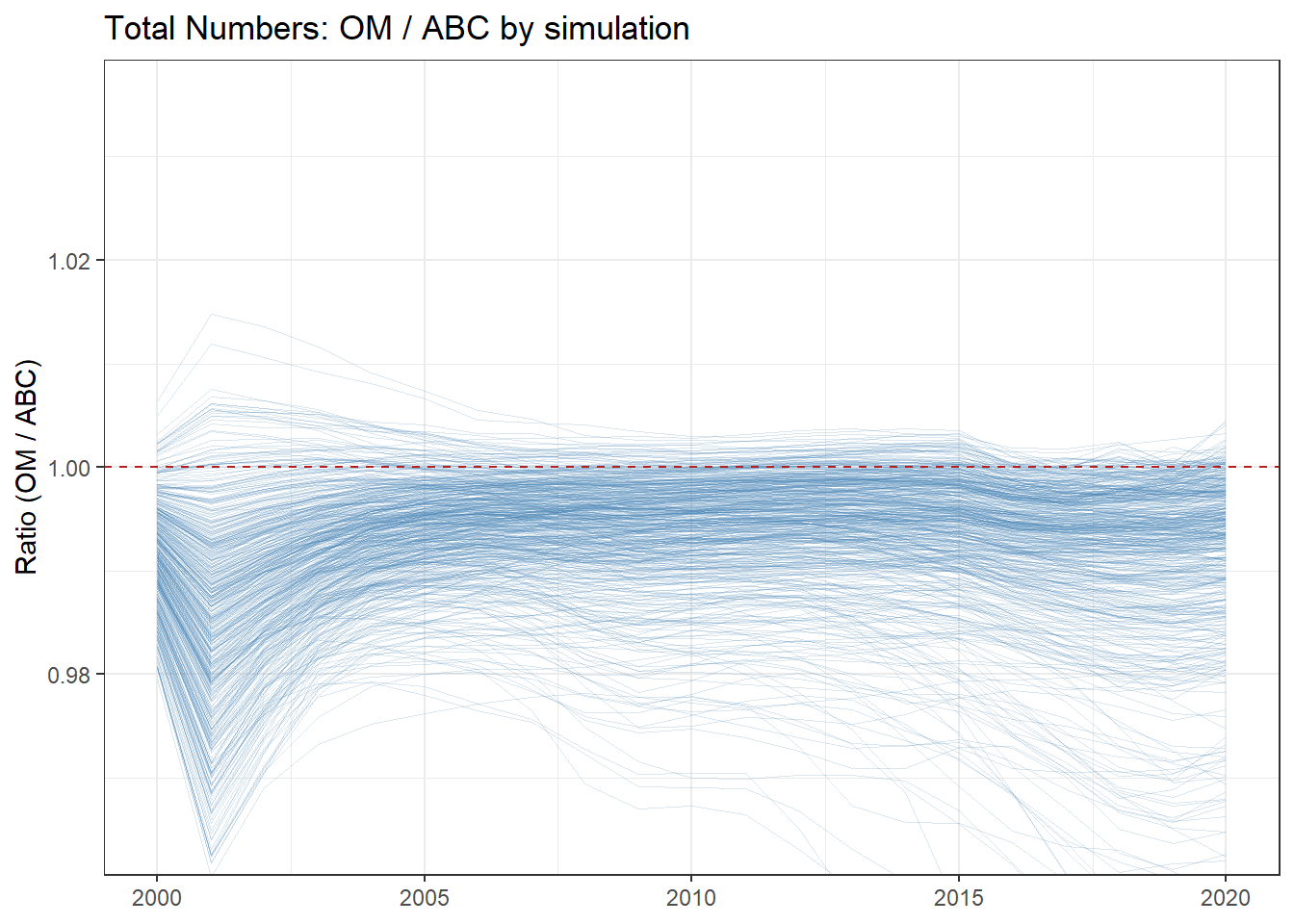
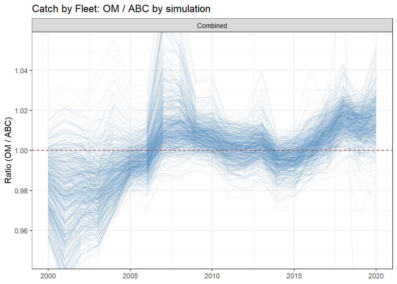
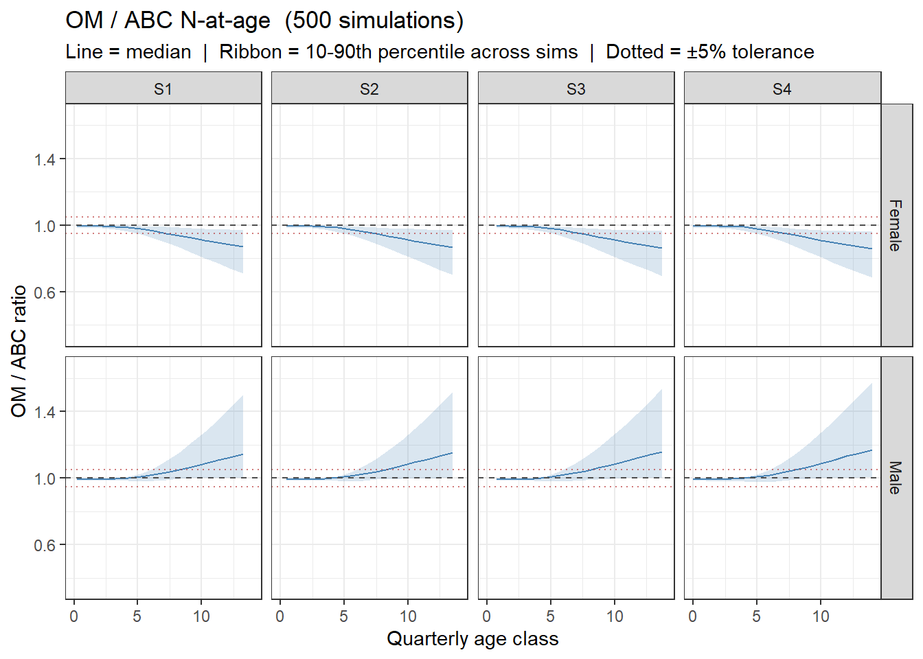
The consequence of this difference in model structure is that the OM can deviate from the conditioning model by up to approximately 5% in numbers for most simulations, with a small number of simulations (those characterised by high exploitation rates or extreme stock-recruit parameters) diverging by up to ~20% in the final years of the historical period (Section 2.4.2).
The choice between harvest rate and instantaneous F reflects an assumption about how fishing activity actually occurs in time. The harvest rate (pulse) approach is more appropriate when fishing is concentrated into a brief period within the season. The Baranov (continuous) approach is more appropriate when fishing effort is spread continuously throughout the season.
2.4.2 Comparison with the Conditioning Model
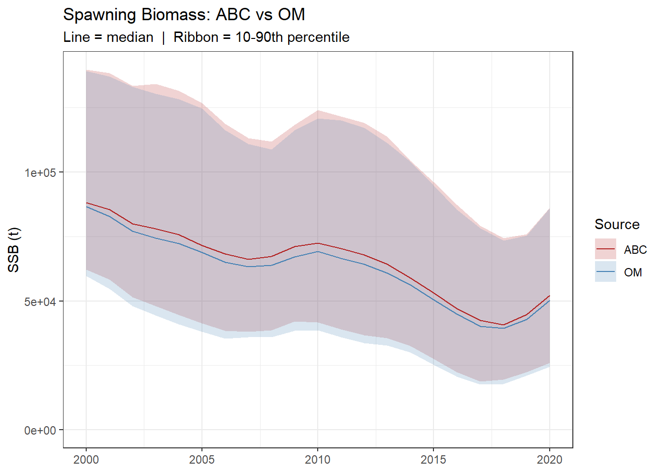
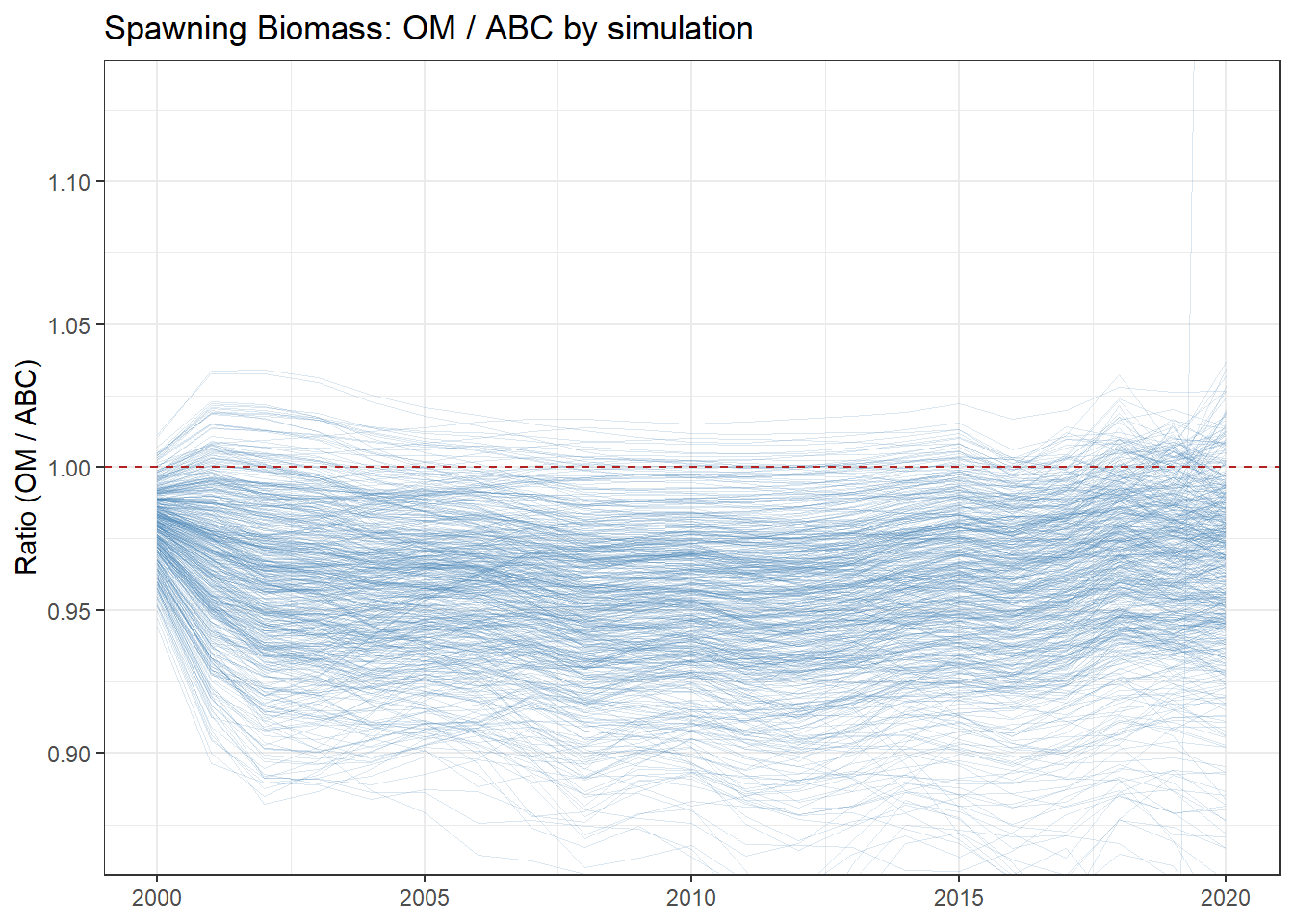
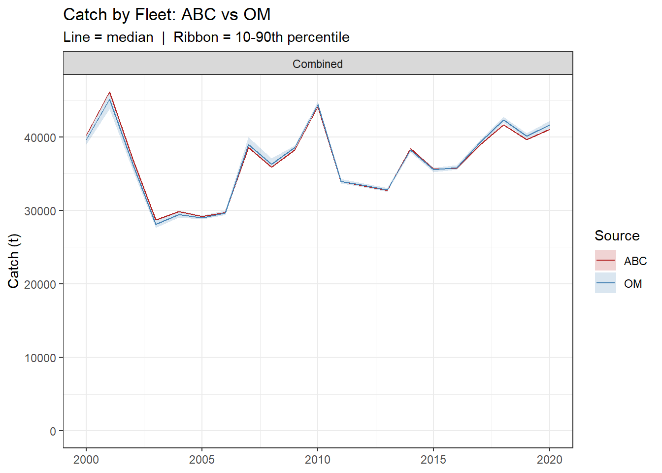
The figures below compare the Base Case OM dynamics against the ABC conditioning model across the 500 MCMC simulations. In each ribbon plot, the line shows the posterior median and the shaded band the 10th–90th percentile interval for the ABC model (red) and the OM (blue). The ratio plots show OM / ABC for each individual simulation, with the dashed red line at 1 indicating perfect agreement. Catch is compared for the total of the six fleets, as these are combined in the OM.
2.4.2.1 Total Numbers
2.4.2.2 Spawning Biomass
2.4.2.3 Catch
2.4.2.4 Numbers-at-Age
2.4.3 Potential Remedies
Two options exist to resolve the discrepancy between the conditioning model and the OMs used in the MSE:
Extension of the
openMSEframework to support pulse fishing. It is technically possible to implement a harvest rate option within theopenMSEframework to replicate the ABC model dynamics exactly. However, this represents a non-trivial software development effort requiring changes to the core simulation engine, and is considered outside the scope of the present project.Reconditioning the ABC model using instantaneous F. An alternative remedy is to convert the ABC conditioning model to use the Baranov catch equation and recondition the model on the available data.
The decision of whether to reconcile these differences, and which approach to pursue, will be made collaboratively by the managers and scientists involved in this MSE process. At present, the discrepancy between the two approaches is considered acceptable for the purposes of this MSE: the median trajectory of the OM closely tracks that of the ABC model across all key stock dynamic quantities, and the parameter uncertainty captured across simulations substantially exceeds the bias introduced by the harvest rate conversion (Section 2.4.2).