5 Candidate Management Procedures
The MSE currently includes four types of candidate management procedure (CMP), all using the LL1 (NW) CPUE index:
- Index Rate (IR): the TAC is a catch/index rate multiplied by the current index, with the rate reduced by a harvest control rule (HCR) at low stock status;
- Index Target with a Buffer HCR (ITB): the TAC is a reference catch scaled by the ‘buffer’ HCR of the earlier albacore MSE work (Mosqueira & Hillary, 2025);
- Buffer MP (BUF): a replica of the CPUE + buffer HCR MP of the earlier albacore MSE work (Mosqueira & Hillary, 2025), in which the HCR adjusts the previous TAC;
- Surplus Production (SP): the TAC is set from the stock status and FMSY estimated by a surplus production model.
Each CMP type is tuned to two different tuning levels, representing two sets of management objectives (see Section 5.9):
- T1: a probability of being in the Kobe green quadrant;
- T2: the same probability and a probability of never falling below the limit reference point, with larger TAC decreases allowed.
Each CMP is named by its type and tuning level; e.g., IR_T2 is the Index Rate CMP tuned to T2.
All CMPs limit increases in the TAC between management cycles to 15%. Decreases are limited to 15% in the T1 CMPs and 30% in the T2 CMPs (Section 5.8). Variants with a symmetric 30% limit were explored in preliminary runs, where they gave little or no increase in catch with more variable TACs, and were not retained.
All CMPs set a single TAC for the total catch (removals, in t) of all fleets. The CMPs use data aggregated to calendar years: annual catches (summed over the quarters) and annual CPUE indices (averaged over the quarters with data).
5.1 Estimated Stock Status
The index-based CMPs estimate stock status from the LL1 CPUE index. The index is expressed relative to its level at SBMSY, IMSY, calculated from the mean index over 2016–2020 and the median (over simulations) of the mean SB/SBMSY over the same years in the Base Case OM (1.75):
\[I_{\text{MSY}} = \frac{\bar{I}}{\overline{SB/SB_{\text{MSY}}}} \tag{5.1}\]
giving IMSY = 0.411.
The current status of the index, \(S\), is the index averaged over the most recent years, after optional loess smoothing (the number of years and the smoothing are CMP settings; Section 5.9). The estimated stock status, in units of SB/SBMSY, is \(x = S / I_{\text{MSY}}\).
The Surplus Production CMPs estimate stock status as the estimated biomass relative to BMSY at the start of the year the TAC applies (Section 5.6).
5.2 Harvest Control Rules
The HCRs are specified in terms of estimated stock status relative to SBMSY (or BMSY), with the limit reference point (LRP; 0.4 SBMSY) as a control point (IOTC, 2015).
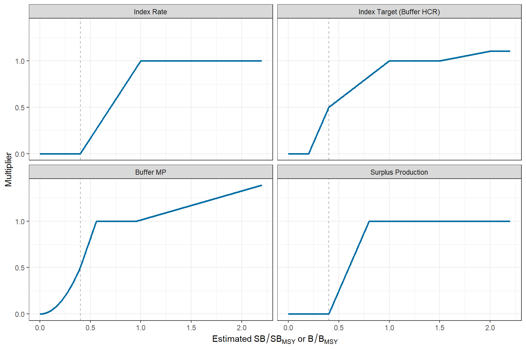
The output of each HCR is a multiplier on a quantity specific to each CMP type, from which the TAC is calculated (Figure 5.1):
- Index Rate: the catch/index rate;
- Index Target with a Buffer HCR: a reference catch;
- Buffer MP: the previous TAC;
- Surplus Production: FMSY estimated by the surplus production model.
The intensity of fishing is set by the tuning parameter (Section 5.9).
The HCRs of the Index Rate and Surplus Production CMPs act on a harvest rate (the catch/index rate or the fishing mortality), so the TAC follows the stock, and the fishing intensity is reduced as the estimated stock status declines below the threshold. The HCRs of the Index Target with a Buffer HCR and Buffer MP CMPs act on the TAC itself. These are the buffer MPs of the earlier work, designed to keep the TAC stable while the index is within the buffer, with sharp reductions in the TAC below the lower buffer and the limit.
5.3 Index Rate
The Index Rate CMPs set the TAC as a catch/index rate multiplied by the current index. The catch/index rate, \(\hat{r}\), is the mean total catch over the last 2 historical years divided by the mean index over the same years. The trial TAC is:
\[\text{TrialTAC} = m \times \hat{r} \times S \times \theta(x) \tag{5.2}\]
where \(m\) is the tuning parameter and \(\theta(x)\) is the HCR multiplier: 0 at and below the LRP, increasing linearly to 1 at SBMSY, and 1 above (Figure 5.1). Because the catch/index rate is calibrated to the recent catch, \(m\) = 1 corresponds to the recent catch/index ratio.
The Index Rate CMPs use current status calculated from the index averaged over the most recent year after loess smoothing (Section 5.9).
5.4 Index Target with a Buffer HCR
The Index Target with a Buffer HCR CMPs set the TAC as a reference catch, the mean total catch over the last 5 historical years (\(\bar{C}\)), scaled by the tuning parameter and the HCR:
\[\text{TrialTAC} = m \times \bar{C} \times \theta_C(x) \tag{5.3}\]
The HCR, \(\theta_C(x)\), has the shape of the buffer HCR of the earlier albacore MSE work (Mosqueira & Hillary, 2025) (Figure 5.1):
- 1 (the reference catch) between the lower and upper buffers (1 and 1.5 SBMSY);
- decreasing linearly below the lower buffer to 0.5 at the LRP, and more rapidly below the LRP, to zero at 0.2 SBMSY;
- increasing above the upper buffer at a quarter of the rate of the decrease between the LRP and the lower buffer, to 1.1 at 2 SBMSY.
The output is applied to a fixed reference catch (the first formulation tested in the earlier work), so the TAC remains stable while the index is between the buffers, and the reference catch is the tuning parameter. The position of the buffers is a CMP setting (Section 5.9).
The Index Target with a Buffer HCR CMPs use current status calculated from the index averaged over the most recent year, and buffers at 1 and 1.5 SBMSY (Section 5.9).
5.5 Buffer MP
The Buffer MP CMPs replicate the CPUE + buffer HCR MP of the earlier albacore MSE work (Mosqueira & Hillary, 2025). In each management cycle, the MP calculates an index metric, applies the buffer HCR to it, and multiplies the previous TAC by the output of the HCR.
The index metric, \(x\), is a weighted mean of the LL1 index over the last 4 data years, relative to its level at SBMSY (IMSY; Section 5.1):
\[ x = \frac{1}{I_{\text{MSY}}} \sum_{i=1}^{4} w_i \, I_{y_i} \tag{5.4}\]
where \(y_1, \ldots, y_4\) are the last four data years, from the oldest to the most recent. The most recent year has a weight of 0.5, and the other 0.5 is shared among the three earlier years in proportion to their position (1, 2, and 3), giving weights of \(w_i\) = 1/12, 2/12, 3/12, and 6/12. The metric therefore responds mainly to the most recent index value, with some smoothing from the earlier years. For example, the first TAC (2029) uses the index in 2023–2026, with the highest weight on 2026.
The HCR multiplier, \(\theta_B(x)\), is (Figure 5.1):
\[ \theta_B(x) = \begin{cases} \dfrac{1}{2}\left(\dfrac{x}{L}\right)^2 & x \le L \\[8pt] \dfrac{1}{2}\left(1 + \dfrac{x - L}{B_1 - L}\right) & L < x \le B_1 \\[8pt] 1 & B_1 < x < B_2 \\[4pt] 1 + s \dfrac{0.5}{B_1 - L}(x - B_2) & x \ge B_2 \end{cases} \tag{5.5}\]
where \(L\) is the limit, \(B_1\) and \(B_2\) are the lower and upper buffers, and \(s\) is the ratio of the slope of the increase above the upper buffer to the slope of the decrease between the limit and the lower buffer.
The TAC is the previous TAC multiplied by the HCR output:
\[ \text{TrialTAC} = \text{TAC}_{\text{prev}} \times \theta_B(x) \tag{5.6}\]
The TAC is therefore held while the index metric is between the buffers, reduced in every management cycle while it is below the lower buffer, and increased in every management cycle while it is above the upper buffer. Unlike the other CMPs, changes in the TAC of less than 1% are not ignored (Section 5.8).
As in the earlier work, the CMP is tuned by the position of the upper buffer, which is set to \(B_1 + (B_2 - B_1)/m\), where larger values of the tuning parameter \(m\) move the upper buffer towards the lower buffer, so that the TAC increases at lower values of the index and the catch is higher. The tuning parameter does not change the lower buffer or the limit, which determine how quickly the TAC is reduced.
5.6 Surplus Production
Model-based MPs combining a surplus production model with an HCR were also proposed in the earlier albacore MSE work (Mosqueira & Hillary, 2025, 2026). The Surplus Production CMPs fit a Schaefer surplus production model to the annual total catch and the annual LL1 CPUE index from 2000. FMSY and MSY are estimated, the catchability and the observation standard deviation of the index are estimated at their maximum likelihood values, and the catch is assumed known.
To match the dynamics of the Base Case OM, the initial depletion is fixed at the Base Case OM value, and informative priors are used for FMSY and MSY (Table 5.1). The surplus production model has a single biomass pool, so the OM quantities are calculated for the total biomass of both sexes:
- Initial depletion: the median total biomass relative to unfished at the start of 2000;
- FMSY prior: lognormal, with median equal to the median harvest rate at MSY (MSY / BMSY) of the Base Case OM;
- MSY prior: lognormal, with median equal to the median MSY of the Base Case OM.
The CVs of the priors are the CV of the OM values over simulations, or a minimum of 0.3 (FMSY) and 0.4 (MSY), so the priors are informative but allow the data to update the estimates.
In each management cycle, the model is fitted to the available data, starting from the estimates of the previous management cycle, and projected to the start of the year the TAC applies, assuming the catch in the intervening years is the TAC in force. The fishing mortality is:
\[F = m \times \hat{F}_{\text{MSY}} \times \theta\!\left(\hat{B}/\hat{B}_{\text{MSY}}\right) \tag{5.7}\]
where \(m\) is the tuning parameter and \(\theta\) is the HCR multiplier: 0 at and below the LRP (0.4 B/BMSY), increasing linearly to 1 at the HCR threshold, and 1 above (Figure 5.1). The TAC is the mean annual catch when the model is projected at \(F\) over the 3-year management cycle. If the model fit fails or does not converge, the previous TAC is kept.
The Surplus Production CMPs use an HCR threshold of 0.8 B/BMSY (Section 5.9).
| Parameter | Treatment | Value |
|---|---|---|
| Shape (n) | Fixed (Schaefer) | 2 |
| Initial depletion (B/K) | Fixed | 0.84 |
| FMSY | Estimated, lognormal prior | median 0.199, CV 0.30 |
| MSY (t) | Estimated, lognormal prior | median 51,055, CV 0.40 |
5.7 Input Data When the MP Is Applied
In the MSE, each CMP is applied in every management cycle to the historical catch and CPUE data, plus the observations added since the previous cycle. Once a data value has been observed, it does not change in later management cycles. The performance of the CMPs, and the tuning of their catch level, therefore assume that the MP will be applied in the same way: new data are added to the existing series, but the existing values are not revised.
This matters because the CMPs are calibrated to the historical data. For example, the index level at SBMSY (IMSY), which sets the position of the HCR control points of the index-based CMPs, is calculated from the historical LL1 index (Section 5.1). If the historical index were revised after an MP is adopted, for example by a new standardisation of the CPUE, the same stock status would give a different index relative to IMSY, and therefore a different TAC. The MP applied would then no longer be the MP that was tested. The revision of the historical LL1 index between the 2022 and 2025 stock assessments (Section 2.1.4) shows that revisions of this size can occur.
When an MP is adopted, its specification should therefore include the data it uses:
- The index: The standardisation model, fleets, areas, seasons, and data selection should be fixed, so that new years can be added without changing the historical values (for example, by fixing the historical index and scaling new values to it);
- The catch data: The catch series used by the MP should be defined in the same way;
- A review process: Changes to the input data that cannot be avoided (e.g. revisions to the reported catches, or changes in the fishery that require a new standardisation) should be reviewed by the scientific committee, and may require the MP to be re-calibrated and re-tested in the MSE before it is applied.
5.8 TAC Change Limits
The TAC calculated by a CMP (the trial TAC) is constrained so that it does not change by more than a set proportion from the TAC in force:
\[ \text{TAC} = \text{TAC}_{\text{prev}} \times \min\left(\max\left(\frac{\text{TrialTAC}}{\text{TAC}_{\text{prev}}},\ 1 - \delta_{\text{down}}\right),\ 1 + \delta_{\text{up}}\right) \tag{5.8}\]
where \(\text{TAC}_{\text{prev}}\) is the TAC in force, and \(\delta_{\text{up}}\) and \(\delta_{\text{down}}\) are the maximum proportional increase and decrease. In the first management cycle, \(\text{TAC}_{\text{prev}}\) is the catch in the last initial projection year (Section 3.2). For all CMPs except the Buffer MP, changes of less than 1% are ignored, and the TAC is left unchanged.
The limits differ between the tuning levels:
- T1: TAC increases and decreases are both limited to 15%, as in the earlier albacore MSE work;
- T2: TAC increases are limited to 15%, and TAC decreases to 30%.
The T2 CMPs allow larger decreases because, with a 15% limit, no CMP could meet the safety constraint of T2 (Section 5.9). With a 15% limit, the TAC can fall by at most 15% every 3 years, i.e., to 61% of its initial level after three management cycles. In the simulations where the stock is already depleted by the catches of the initial projection years (Section 3.2.1), this is not fast enough to prevent the stock from falling below the LRP, even if the CMP sets a TAC close to zero.
5.9 Tuning Methodology
Each CMP has a single tuning parameter, \(m\), that scales the target fishing intensity.
The CMPs are tuned for the Base Case OM to maximise the mean annual catch over 2029–2058, subject to the constraints of two tuning levels (Chapter 4):
- T1 (Status): a probability of at least 0.6 of being in the Kobe green quadrant over 2044–2058 (the proportion of simulations and years);
- T2 (Status and Safety): the T1 constraint, and a probability of at least 0.9 that spawning biomass stays above the LRP (0.4 SBMSY) in every year over 2034–2058. A simulation in which spawning biomass falls below the LRP in any year is a breach, so at most 10% of simulations may breach the LRP. The T2 CMPs allow TAC decreases of up to 30% (Section 5.8).
The two tuning levels show the trade-off between catch and the risk of depleting the stock. In preliminary runs, maximising the catch subject only to the probability of the Kobe green quadrant (T1) led to CMPs that depleted the low-productivity simulations (low MSY; Section 2.2) to well below the LRP, while the probability of the Kobe green quadrant, averaged over all simulations and years, was kept at its minimum by the other simulations. The safety constraint of T2 limits the proportion of simulations where this happens.
The safety constraint excludes the first 5 years the CMPs are active (2029–2033), one management cycle and two years, so that the stock can recover from the catches in the initial projection years, which the CMPs do not control (Section 3.2).
The CMPs were tuned with 80 of the 500 simulations. The 80 simulations were a stratified random sample where the simulations were split into 8 groups of equal size by MSY, and each group then split into 10 groups of equal size by female SB/SB0 in 2020, and one simulation drawn from each group. The tuning simulations therefore have the same distribution of productivity and stock status as all simulations, including the simulations where the stock collapses before the CMPs start (Section 3.2.1).
The tuning is done in two steps.
5.9.1 Step 1: CMP Settings
In addition to the tuning parameter \(m\), the Index Rate, Index Target with a Buffer HCR, and Surplus Production CMPs have other settings that affect their performance, including for example the number of years used to calculate the current index (Table 5.2). For each of these CMP types, the settings were chosen from a small set of candidate values, as the configuration of values that gives the highest catch when the CMP is tuned to the T1 constraint:
- Each configuration was projected at 5 values of \(m\) over 0.1–3, using 40 of the tuning simulations, and the catch at the value of \(m\) that meets the constraint was interpolated;
- The configuration with the highest catch was then fully tuned (Step 2) with all 80 tuning simulations.
The selected settings are used for the CMPs of that type at both tuning levels. The Buffer MP CMPs use the settings of the earlier work, so no settings were selected for them.
| Setting | Candidate values | Selected |
|---|---|---|
| Index Rate | ||
| Years averaged for current status | 1, 3 | 1 |
| Index smoothing | yes, no | yes |
| Index Target (Buffer HCR) | ||
| Years averaged for current status | 1, 3 | 1 |
| Lower and upper buffer (SB/SBMSY) | 0.8–1.2, 1–1.5 | 1–1.5 |
| Surplus Production | ||
| HCR threshold (B/BMSY) | 0.8, 1 | 0.8 |
5.9.2 Step 2: Tuning Parameter
\(m\) was then tuned for each of the 8 CMPs (4 CMP types at 2 tuning levels). It was first evaluated on a grid of 7 log-spaced values over 0.1–3, which was extended by a factor of 3 up to 3 times if necessary, and then refined towards the largest value that meets the constraints (or the value with the highest catch, if that is lower), until the range of \(m\) is within 1% or the binding constraint is within 0.5% of its minimum (Table 5.3). A CMP for which no value of \(m\) meets the constraints is reported as infeasible and is not projected.
| CMP | m | Mean catch (t) | P(Kobe green) | P(SB > LRP every year) |
|---|---|---|---|---|
| T1 (TAC decreases of up to 15%) | ||||
| IR_T1 | 1.59 | 43,808 | 0.60 | 0.68 |
| ITB_T1 | 1.18 | 40,770 | 0.60 | 0.70 |
| BUF_T1 | 0.21 | 41,811 | 0.60 | 0.66 |
| SP_T1 | 1.01 | 43,577 | 0.60 | 0.61 |
| T2 (TAC decreases of up to 30%) | ||||
| IR_T2 | 1.29 | 39,617 | 0.82 | 0.90 |
| ITB_T2 | 0.86 | 33,384 | 0.86 | 0.90 |
| BUF_T2† | – | – | – | – |
| SP_T2 | 0.63 | 33,424 | 0.88 | 0.90 |